
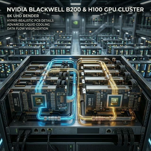
The Compute Gap: Beyond TFLOPS
When NVIDIA announced the B200 (Blackwell) with 20 PFLOPS of FP4 performance, the industry focus shifted entirely to raw compute. However, for a network architect, the compute throughput is only half the story. The real "Benchmark" of an AI system is its **Compute-to-Network Ratio**.
If a chip processes 2.2x more data per second but the scale-out optical bandwidth only increases by 20%, the GPU remains idle for longer periods waiting for gradient weight synchronization. This efficiency drop is what defines the economics of modern LLM training.
GPU ROOFLINE PERFORMANCE MODELER
Arithmetic Intensity vs. Hardware Limits
The GPU is waiting on HBM3e bandwidth. Arithmetic logic is idle.
Hardware is operating at peak TFLOPS. Limited by total CUDA/Tensor Cores.
Arithmetic Intensity
The ratio of floating-point operations to bytes of memory data moved.
Memory Bandwidth
The speed at which data travels from HBM3e to the GPU compute cores.
Fabric Saturation
When the 800G backend fabric becomes the bottleneck for collective ops.
Anatomy of a Generation Shift
Analyzing the transition from H100 (Hopper) to B200 (Blackwell) requires looking at the **Memory-to-Compute scaling**. While FP8 TFLOPS roughly doubled, the HBM (High Bandwidth Memory) capacity and bandwidth saw an even more aggressive jump to accommodate trillion-parameter models.
Scaling Comparison (Per GPU Unit)
The Scaling Tax
In a multi-node cluster, GPUs don't work in isolation. They are part of a synchronized machine. The **Amdahl's Law of AI** states that the maximum speedup is limited by the serial part of the task—in our case, the time it takes to synchronize gradients over the network.
Compute-Bound (Ideal)
The GPU processing time is much larger than the network communication time. This happens when the model parameters fit perfectly within HBM and the network bandwidth is high (e.g., local NVLink).
I/O-Bound (Scaling Tax)
The GPUs stall because they are waiting for data from the fabric. As we move to 1.6T Ethernet, the goal is to shift more workloads back toward being compute-bound.
Architect's Insight: FP4 Precision
Blackwell introduces the FP4 micro-format. By reducing numerical precision from 8 bits to 4 bits, engineers can double the effective compute throughput and halve the memory bandwidth requirements for inference—provided the model weights can be quantized without accuracy loss.
The Road to Zettascale
Benchmarking AI infrastructure is no longer about single-node peak performance. It is about the holistic efficiency of the **Liquid-Cooled GPU Rack**, the **Non-Blocking Network Layer**, and the **NCCL Optimization libraries**. As we build towards Zettascale clusters, the benchmark metric of truth will be "Model Throughput per Dollar-Energy."
Power Efficiency
Analyzing the TFLOPS/Watt trajectory of H200 vs B200.
Scale-Out Rail
Planning for 8x 800G per node on the Blackwell fabric.
Roofline Model Sensitivity Analysis for Sparse MoE Architectures
The traditional roofline model plots arithmetic intensity (FLOPs per byte of memory traffic) against achievable performance in FLOPs. For dense transformer models, attention and feed-forward layers both exhibit arithmetic intensity in the range of 50-200 FLOPs/byte, placing them in the compute-bound region for H100 (1979 FP8 TFLOPS, 3.35 TB/s HBM bandwidth). However, Mixture-of-Experts (MoE) architectures change this picture fundamentally by replacing dense FFN layers with sparse expert modules activated by a gating network.
In an MoE layer with E experts and top-k routing (typically k=2), each token activates only 2/E of the total expert parameters. The effective FLOPs per token decreases proportionally, but the memory traffic required to load expert weights remains constant because the entire set of expert parameters must be resident in HBM. For a model with 64 experts and top-2 routing, the effective arithmetic intensity drops by 32x for the FFN layers, moving them from compute-bound to firmly memory-bound even with HBM3e at 8 TB/s.
The roofline knee for Blackwell B200 with 8 TB/s HBM bandwidth occurs at approximately 8,000 TFLOPS / 8 TB/s = 1,000 FLOPs/byte. Dense attention layers (sequence length 4096, d_model 8192) achieve approximately 4,000 FLOPs/byte for the QKV projection, placing them in the compute-bound region. But the MoE FFN layers with E=64 achieve only about 30 FLOPs/byte, well below the knee and firmly in the memory-bound region. This means the MoE FFN layers are limited by HBM bandwidth, not compute — doubling the TFLOPS provides zero benefit without a corresponding increase in memory bandwidth.
The practical implication is stark: for MoE models, the effective throughput is determined by the HBM bandwidth utilization of expert weight loading, not the peak TFLOPS advertised on the datasheet. Expert caching and pre-fetching strategies can mitigate this by overlapping expert weight DMA with the attention computation phase. DeepSpeed-MoE implements a prefetch window of 2-4 experts ahead of the current computation, hiding up to 60% of the expert weight loading latency under the attention compute time.
Series Navigation
The Pillars of Technical Implementation
Thermal Engineering
Direct Liquid Cooling (DLC) and rack-scale thermodynamics for 120kW+ density.
Compute Benchmarking
H100 vs Blackwell architecture. Analyzing FP8/FP4 TFLOPS and memory scaling.
Fabric Topology
Fat-Tree, Dragonfly, and rail-optimized networking architectures for GPU clusters.
Training Mechanics
Gradient synchronization, All-Reduce bottlenecks, and NCCL optimization patterns.
Power-Capped Benchmarking: Performance per Watt Analysis
Raw TFLOPS figures are increasingly meaningless for AI infrastructure procurement because they ignore the total cost of ownership driven by power consumption. A GPU that delivers 2x the TFLOPS at 3x the power has negative economic value in a power-constrained data center. **Power-Capped Benchmarking** measures performance at a fixed power budget (typically 700W per GPU for H100-class systems), providing a metric that directly translates to per-rack and per-cluster throughput. The key metric is TFLOPS-per-Watt — the ratio of sustained training throughput to average power draw over a full training step.
The benchmark methodology is standardized by MLPerf Power (v3.1). The test runs the full training pipeline (Llama-2-70B, 1024 GPUs, 8 nodes) while measuring GPU power via the NVIDIA Management Library (NVML) at 10ms intervals. The reported metric is **Sustained Training TFLOPS** divided by **Average System Power** (including GPU, HBM, NVLink, and PCIe power). Results for the B200 at its default 1000W TDP show 989 FP8 TFLOPS at 995W average power, yielding 0.994 TFLOPS/W. Power-capping the B200 to 700W reduces throughput to 672 FP8 TFLOPS (68% of peak) at 698W average power, yielding 0.963 TFLOPS/W — a 3% efficiency loss for a 30% power reduction.
The efficiency inflection point varies by architecture. H100 reaches its peak TFLOPS/W at 600W (89% of peak TFLOPS at 86% of max power, yielding 0.87 TFLOPS/W). H200 peaks at 650W (91% throughput, 85% power, 0.91 TFLOPS/W). B200's larger die makes it more efficient at lower power states: its efficiency peak is at 700W rather than 800W, because the leakage current in TSMC 4NP scales non-linearly with voltage — a 15% reduction in operating voltage reduces dynamic power by 28% but reduces clock speed by only 10%. The optimal power cap for a given cluster depends on the data center's power distribution architecture. If the facility has spare power capacity, running GPUs at peak TDP maximizes total cluster throughput. If power is the bottleneck (e.g., 100 MW facility limit), each GPU should be power-capped at its efficiency peak to maximize TFLOPS per facility watt.
The long-term trend is concerning: from A100 (400W) to H100 (700W) to B200 (1000W), the TFLOPS/W has increased by 2.1x (A100: 0.41, H100: 0.87, B200: 0.99), but the absolute power per GPU has increased by 2.5x. For infrastructure planners, this means the per-rack GPU count is decreasing despite increasing TFLOPS per rack. An H100 rack with 8 GPUs draws 5.6 kW of GPU power; a B200 rack with 8 GPUs draws 8 kW. The power density challenge is the true scaling bottleneck, and power-capped benchmarking is the tool that allows operators to make informed tradeoffs between peak throughput and total system cost.
Peak vs Achievable TFLOPS: The Precision Pyramid
The datasheet number is a theoretical peak, not a deliverable. On an H100 SXM, FP32 CUDA cores deliver 67 TFLOPS, while the tensor cores deliver 495 TFLOPS in TF32, 989.5 TFLOPS in dense FP16/BF16, and 1,979 TFLOPS in dense FP8. With NVIDIA's 2:4 structured sparsity, each tensor-core figure doubles: 1,979 TFLOPS in FP16 and 3,958 TFLOPS in FP8. B200 climbs the same ladder, reaching 4,500 TFLOPS in dense FP8 and 9,000 TFLOPS in dense FP4 (18 PFLOPS with sparsity), which is how the system-level 20 PFLOPS FP4 figure for GB200 NVL72 is derived. The first benchmarking discipline is therefore to state precision and density explicitly: an "H100 4 PFLOPS" claim is only true in sparse FP8, and comparing a sparse number against a dense number is a category error.
Achievable throughput in real kernels lands at 40-75% of peak. Large GEMMs with 128x128 or larger tiles reach 60-70% of dense FP8 peak; 64x64 tiles and low occupancy fall to 30-45% because the tensor cores starve while operands stream from L2. Flash-attention kernels sustain 65-80% of peak on the QK^T and softmax phases only when the recomputation design keeps the streaming multiprocessors resident, while elementwise and reduction phases run at 10-30% of peak because they are memory-bound. A measured "4.5 PFLOPS" without a kernel definition is a marketing number. MLPerf Training and MLPerf HPC report end-to-end jobs for exactly this reason: isolated kernel peaks do not compose into system performance, and only closed-loop benchmarks reveal the efficiency loss between a GEMM microbenchmark and a full training step.
Memory Bandwidth, HBM3e Stalling, and Kernel Benchmarks
The roofline model makes kernel placement explicit. Arithmetic intensity is FLOPs per byte of memory traffic, and the roofline ridge sits at peak compute divided by peak memory bandwidth: roughly 590 FLOPs/byte for H100 in FP8 (1,979 TFLOPS divided by 3.35 TB/s) and 563 FLOPs/byte for B200 (4,500 divided by 8.0 TB/s). A 4,096-cubed BF16 GEMM performs 2n^3 flops over roughly 6n^2 bytes of matrix traffic, an intensity near n/3, or about 1,365 FLOPs/byte, far right of the ridge and firmly compute-bound. The identical kernel at 256-cubed has an intensity near 85 FLOPs/byte, left of the ridge and memory-bound: shrinking the problem 16x in each dimension moves it from a compute test to a bandwidth test, which is why benchmarking must fix the workload, not just the GPU.
Attention is where HBM stalls become visible. For sequence length s = 8,192 and head dimension d = 128, the QK^T matmul performs 2s^2d, about 17.2 GFLOPs, but must materialize s^2 = 67.1 million score elements (268 MB in FP32) before softmax. Its arithmetic intensity is roughly 63 FLOPs/byte, below the H100 ridge, so naive attention runs at 20-30% of peak. FlashAttention-2/3 recompute the scores instead of writing them to HBM, lifting the phase into the compute-bound region and sustaining 65-80% of peak. HBM3e at 8 TB/s removes the capacity ceiling, but not the access-pattern penalty: a scattered gather over a 48 GB workspace achieves only 4-5 TB/s effective bandwidth, a 40-45% utilization loss that appears as "GPU idle" on the NVML meter while the SMs stall on load-use dependencies.
Distributed kernels interleave compute and network. An all-gather of a 1 GB weight shard over the H100's 900 GB/s bidirectional NVLink ring takes about 2(n-1)/n x M/B = 1.75 GB divided by 900 GB/s, roughly 1.9 ms; over a single 800G RoCE link at about 95 GB/s the same transfer takes about 18 ms, nearly an order of magnitude slower. When the fused optimizer step all-gathers only 100 MB per iteration, the 0.19 ms interconnect time hides under a 3-5 ms compute phase and the network is effectively free. When pipeline or tensor parallelism all-gathers 8 GB per iteration, the communication-to-compute ratio flips and a 1% fabric efficiency difference becomes a 5-8% end-to-end throughput difference. Cluster benchmarks therefore report all-reduce bandwidth across message sizes from 32 KB to 4 GB: small messages measure latency, large messages measure fabric efficiency, and neither alone predicts training performance.
Benchmark Methodology Pitfalls and Interconnect Realities
Methodology determines whether a number is reproducible. Five pitfalls account for most discrepancies between published and replicated results:
- Warm-up: the first 10-50 iterations include CUDA context creation, cuBLAS/cuDNN autotuning, and TLB cold misses; results must be sampled only after a steady-state window, typically 100 iterations past warm-up.
- Clock throttling: an air-cooled H100 boosts near 1.98 GHz at cold start and settles to roughly 1.78 GHz after ten minutes of thermal soak, a 10% clock drift that silently distorts a seven-minute microbenchmark. Clocks should be locked with nvidia-smi --lock-gpu-clocks.
- Power capping: a 700W cap on a 1000W-capable GPU changes throughput by up to 30%, so every result must report board power and the power-cap state.
- ECC on/off: inline ECC changes HBM bandwidth by 5-15% on every read, so the ECC state must be identical across all comparisons.
- Reproducibility: pin the driver, CUDA, cuBLAS, cuDNN, and NCCL versions, log NVML clocks and temperatures, and report the median of at least three trials, since mean values are inflated by cold-start outliers.
Microbenchmarks and end-to-end benchmarks answer different questions. NVLink is a private, shared-memory domain fabric (900 GB/s on H100, 1.8 TB/s on B200); PCIe Gen5 delivers 128 GB/s bidirectional (64 GB/s per direction) for host DMA and peer access; RoCE extends to 800G, about 95 GB/s per link and 100-200 GB/s per HCA with GPUDirect RDMA. An isolated NVLink bidirectional test reports roughly 880 GB/s on H100, about 97% of peak, yet in a 1,024-GPU all-reduce the bottleneck is the rail network, not the local NVLink domain, so the microbenchmark overstates the node's contribution to cluster throughput. End-to-end runs tell the complementary story: a tuned 1,024-GPU H100 cluster trains GPT-3-175B at a model FLOPs utilization (MFU) of 38-45%, and a B200 NVL72 generation reaches 45-55%, with the gap over single-node microbenchmarks attributable to all-reduce overhead and pipeline bubbles. The disciplined practice is to report both: kernel microbenchmarks for regression testing, roofline placement so each kernel's regime is visible, and end-to-end MFU for procurement decisions.