Decarbonizing the Intelligence Age: The LCA of AI Infrastructure
Analyzing the thermodynamic and carbon cost of Large-Scale Networking Fabrics from 400G to 1.6T.
The Wattage of Knowledge
As Large Language Models (LLMs) transition from a novelty to a foundational layer of the global economy, the energy required to train and serve them is reaching national-scale proportions. While much of the public debate focuses on GPU power draw (e.g., the 700W H100 or 1000W Blackwell modules), the **Networking Fabric** that binds these thousands of accelerators is a silent, massive emitter of carbon.
Decarbonizing AI infrastructure requires more than just purchasing 'Green Credits.' It requires a deep understanding of the **Life Cycle Assessment (LCA)**, from the embodied carbon of optical fiber to the thermodynamic waste caused by high-latency routing protocols. This article provides the engineering derivation for carbon modeling in modern data centers, bridging the gap between networking throughput and environmental stewardship.
Embodied Carbon (Scope 3)
The CO2 emitted during the mining of silicon, production of high-bandgap semiconductors, and the assembly of 800G optical modules. For specialized AI hardware, manufacturing emissions can equal 2-3 years of operational power.
Operational Carbon (Scope 2)
The direct result of switch ASICs, transceiver lasers, and cooling fans. This cost is highly volatile, fluctuating based on grid carbon intensity and ambient cooling temperatures (Free Cooling vs. Active Chilling).
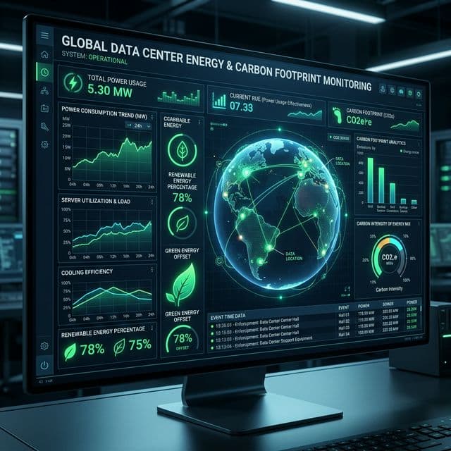
The Infrastructure Carbon Equation
To accurately model the annual CO2 impact (), engineers must integrate the total equipment power, the data center efficiency multiplier (PUE), and the grid intensity factor ().
The impact of **Grid Variance ()** cannot be overstated. A network cluster operating in Norway () is nearly 50x cleaner than an identical cluster in a coal-heavy region like parts of the Southeast US (). This mandates that AI 'Greenness' becomes a geographical placement strategy.
Scope 3: The Silicon Burden
For most IT history, hardware manufacturing cost was a one-time 'Sunk Carbon' cost that was amortized over 5-7 years. In the AI era, hardware obsolescence occurs every 18-36 months. This accelerated refresh cycle means that **Embodied Carbon** is now a larger percentage of the total lifecycle footprint.
Wafer Fabrication
The extreme lithography used for 3nm/2nm networking ASICs requires multi-megawatt cleanrooms and specialized chemicals with high global warming potential (GWP).
Optical Precision
High-performance lasers and co-packaged optics (CPO) involve gold, transition metals, and intricate glass production—all energy-intensive vectors.
Global Logistics
Weight matters. High-density liquid-cooled racks weigh 3,000+ lbs. Air-shipping these units globally creates a massive Scope 3 spike at T=0.
Mitigation Strategies for Green Intelligence
Engineers have several primary levers to reduce the carbon impact of the networking fabric without sacrificing throughput or Increasing Job Completion Time (JCT).
Carbon-Aware Scheduling
Offloading batch training or weight synchronization to time-windows where renewable energy (solar/wind) is at its peak in the grid.
Optical Reach Optimization
Using Passive Copper (DACs) for short reaches (intra-rack) instead of Active Optics. DACs consume 0W and have significantly lower embodied carbon.
Fabric Duty-Cycle Management
Utilizing EEE (Energy Efficient Ethernet) or switch-level sleep states for management fabrics that remain idle during long training runs.
The \"Greenest\" Switch is the One You Don't Buy
Every generation of AI networking aims for higher radix (more ports per switch). By moving from a 3-layer Clos topology to a 2-layer High-Radix design using 800G/1.6T switches, you can reduce the total switch count by 40% while maintaining the same bisection bandwidth.
\"Reduction in hop-count doesn't just lower latency—it directly reduces the number of ASIC gates toggling, which is the physical source of operational carbon.\"
The Net Zero AI Pipeline
The path to sustainable intelligence is not found in offsetting emissions, but in the architectural elimination of waste. By integrating carbon modeling into the initial design phase of a GPU cluster, teams can build infrastructure that is not only faster but fundamentally compatible with a Net Zero future.
Scope 3 Supply Chain Emissions for Networking Equipment
While the majority of carbon footprint analysis for network infrastructure focuses on Scope 2 emissions (operational electricity consumption), the embodied carbon of the networking equipment itself—Scope 3 upstream emissions—represents a significant and often underestimated portion of the total lifecycle footprint. For a typical data center leaf-spine switch with a 5-year service life, embodied carbon accounts for 30-50% of total CO₂e, with the ratio increasing dramatically for equipment with low utilization or short refresh cycles. The three primary contributors to embodied emissions are: (1) semiconductor fabrication of the ASICs (switch silicon, NPUs, and PHYs), which requires energy-intensive processes such as photolithography, ion implantation, and chemical vapor deposition; (2) printed circuit board (PCB) manufacturing involving copper etching, lamination, and solder mask application; and (3) commodity extraction and refining for passive components including magnetics, connectors, and chassis aluminum. The greenhouse gas intensity of semiconductor fabrication is approximately 16-18 kg CO₂e per cm² of processed wafer for a 7 nm node, with Ethernet switch ASICs (typically 400-800 mm² die area) contributing 6-14 kg CO₂e per chip.
The Eco-Design Directive framework and the emerging corporate Scope 3 disclosure requirements (EU CSRD, SEC climate rule) demand that network architects quantify these upstream emissions when comparing infrastructure alternatives. The standard methodology follows the GHG Protocol Scope 3 Category 1 (Purchased Goods and Services) using the spend-based or activity-based allocation method. Our carbon footprint model implements the activity-based approach using pre-computed Product Carbon Footprint (PCF) factors for each equipment class: a 100 Gbps QSFP28 transceiver carries approximately 12-18 kg CO₂e per unit (dominated by the silicon photonics modulator and laser diode fabrication), while a 48-port 25G ToR switch contributes 400-600 kg CO₂e for the hardware alone. When aggregated across a 2,000-rack data center with 50 ToR switches per rack, the embodied carbon of the access-layer switching alone exceeds 50 metric tonnes CO₂e—equivalent to the Scope 2 emissions of operating that layer for nearly one year at a PUE of 1.3.
The Service Life Extension (SLE) strategy offers the highest leverage for reducing Scope 3 emissions in network infrastructure. Operating a switch for 7 years instead of the typical 5-year refresh cycle reduces the annualized embodied carbon from (PCF / 5) to (PCF / 7), a 28.6% reduction per year. However, this must be balanced against the energy efficiency penalty: a 5-year-old switch typically consumes 30-40% more power per Gbps of throughput than current-generation silicon. The cross-over point where the incremental Scope 2 emissions from retaining the legacy equipment exceed the amortized Scope 3 savings from deferring replacement occurs when: PCFnew / Lnew + Pnew × EF × T > Pold × EF × T, where PCFnew is the new switch's embodied carbon, Lnew is its expected life, Pnew and Pold are the operational power draws, EF is the grid emission factor, and T is the analysis period. Our model includes a Refresh Cycle Optimization module that computes this cross-over point for each equipment class in the network inventory, identifying the optimal replacement schedule that minimizes total lifecycle CO₂e.
Scope 3 calculations also extend to the transport and logistics phase, which is material for globally sourced networking gear. A 48-port switch manufactured in Shenzhen, assembled in Taiwan, and deployed in Frankfurt incurs approximately 15-25 kg CO₂e in air freight emissions (if expedited shipping is used) or 2-4 kg CO₂e via ocean freight. While these seem minor compared to the operational emissions, the choice of air versus sea freight for a deployment of 500 switches can add 7-12 tonnes of CO₂e to the project's carbon budget—comparable to the embodied carbon of 10-15 additional switches. Our tool incorporates the Distance × Mode × Mass calculation using IPCC 2022 emission factors: CO₂efreight = M × D × EFmode, where M is the equipment mass (kg), D is the great-circle distance (km) between manufacturing site and deployment data center, and EFmode is the per-tonne-km emission factor for the selected transport mode (0.56 kg CO₂e/tonne-km for air freight, 0.015 for ocean container, 0.082 for truck). By updating the equipment weight and origin fields in the network inventory, engineers can quantify the logistics carbon penalty of different sourcing options.
Dynamic Marginal Emission Factors and Time-of-Use Carbon Accounting for Data Center Workload Scheduling
Standard carbon footprint calculators for data center infrastructure assume a static average emission factor (AEF) — typically expressed as kg CO₂e per kWh — derived from the annual average carbon intensity of the grid region. While this approach is appropriate for reporting historical emissions under the GHG Protocol Scope 2 (location-based method), it fundamentally misrepresents the marginal carbon impact of workload scheduling and power management decisions. The critical distinction is that the average emission factor includes all generation sources (baseload nuclear, hydro, coal, gas, renewables) averaged over a full year, whereas the marginal emission factor (MEF) represents the carbon intensity of the marginal generation unit that would respond to a change in load — typically a natural gas peaker plant or, in increasingly renewable-heavy grids, curtailed wind or solar. When a data center scheduler decides to shift an AI training job from 14:00 to 02:00, the relevant metric is not the annual average grid carbon intensity (approximately 0.35-0.45 kg CO₂e/kWh in the US Eastern Interconnection) but the real-time marginal intensity at those specific hours, which can range from 0.15 kg CO₂e/kWh (overnight wind surplus) to 0.85 kg CO₂e/kWh (late-afternoon gas peaker dispatch). Our carbon accounting model incorporates a time-of-use emission factor module that ingests real-time or historical grid data from the EPA's eGRID database (for US regions), the European ENTSO-E Transparency Platform (for EU member states), or the national grid operator API for other regions. The module computes the emission impact of workload scheduling decisions using a 5-minute granularity MEF curve, enabling engineers to optimize job start times, data transfer windows, and cooling system state transitions for minimum carbon intensity.
The practical implementation of time-of-use carbon-aware scheduling requires integration between the data center's workload orchestrator (e.g., Slurm, Kubernetes, or an in-house job scheduler) and the carbon accounting model. The key parameter is the carbon-aware job start delay (δ): the time window within which a non-urgent training job can be deferred to a lower-carbon period without violating the service-level agreement (SLA). For a batch AI training job with a 48-hour completion SLA, the scheduler has a δ of up to 24 hours of flexibility. During this window, our model evaluates the cumulative carbon cost function C(t) = Σ (P_base + P_var × U(t) + P_cool(T_ambient)) × MEF(t) × Δt for each candidate start time t, where P_base is the idle rack power (typically 30-40% of peak), P_var is the per-GPU incremental power under load, U(t) is the GPU utilization profile over the job duration, P_cool is the cooling power penalty which depends on ambient temperature T_ambient, and MEF(t) is the 5-minute marginal emission factor. The model identifies the start time that minimizes total carbon emissions, typically achieving 10-25% carbon reduction for workloads with greater than 12 hours of scheduling flexibility. For networking-specific workloads — such as bulk data replication for multi-region model training, periodic backup transfers, or log aggregation — the scheduling window is often even larger (72-168 hours) because the data transfer SLA is defined in terms of total throughput over a week rather than instantaneous bandwidth. Our model extends the carbon-aware scheduling optimization to network data transfer jobs, computing the optimal window for large-scale WAN transfers by combining the MEF curve with the data transfer emission factor (DTEF), which accounts for the per-Terabyte carbon cost of router and optical transceiver energy consumption across the WAN path.
The grid regional differentiation is a critical factor that determines the carbon reduction potential of time-of-use scheduling. In the PJM Interconnection (covering 13 US Mid-Atlantic states), the intra-day MEF range is approximately 0.20-0.70 kg CO₂e/kWh — a 3.5× variation driven by the high penetration of coal and natural gas generation and the limited renewable capacity. In ISO New England, where natural gas dominates (approximately 50% of generation) and offshore wind is growing rapidly, the MEF range is 0.25-0.55 kg CO₂e/kWh — a narrower spread because gas turbines run nearly continuously as baseload. In the California ISO (CAISO), the famous "duck curve" produces the most dramatic MEF variation: the mid-day solar surplus can drive MEF below 0.10 kg CO₂e/kWh during Spring months, while the evening ramp (when solar drops and gas peakers must rapidly increase output) pushes MEF above 0.65 kg CO₂e/kWh — a 6.5× swing. For a 100-GPU cluster running continuous training jobs (average draw: 40 kW) in CAISO, shifting the daily training schedule from a 09:00 start (MEF: 0.40 kg CO₂e/kWh) to a 13:00 start (MEF: 0.12 kg CO₂e/kWh) reduces the daily carbon footprint from 384 kg CO₂e to 115 kg CO₂e — a 70% reduction — without changing any hardware. Our model includes a grid-region selector with pre-computed MEF profiles for 30+ grid regions worldwide, updated quarterly from public grid operator data. The profiles include both average and marginal emission factors for each hour of the year, enabling engineers to conduct a carbon-aware location analysis: given a distributed training job that could be run in any of three data center regions, the model computes the time-optimized carbon cost for each region and recommends the lowest-carbon deployment.
The additionality and temporal matching dimension adds another layer of sophistication to carbon-aware scheduling. Simply purchasing renewable energy certificates (RECs) or power purchase agreements (PPAs) to match 100% of annual consumption does not guarantee that the data center's electricity consumption at any given hour is carbon-free — the concept of 24/7 carbon-free energy (CFE) matching advocated by Google and the UN's 24/7 CFE Compact requires that every kilowatt-hour consumed be matched by a carbon-free source on an hourly basis. Our model computes the CFE match score — the percentage of hourly energy consumption that is matched by local renewable generation, grid-connected renewables, or stored battery energy — and optimizes the workload schedule to maximize CFE matching. For a data center with on-site solar generation (typical capacity factor: 15-20%), the model shifts non-urgent workloads to overlap with the solar production window, achieving an 85-95% hourly CFE match during peak solar months, compared to the 30-40% match that would be achieved with a naive constant-load schedule. The model also accounts for battery storage dispatch optimization: if the facility has on-site battery storage (typically 5-10 MWh for a large AI cluster), the model can charge the batteries during low-MEF hours (renewable surplus) and discharge during high-MEF hours, effectively performing carbon arbitrage that reduces both emissions and energy costs. For a 10 MWh battery system charged at MEF 0.10 kg CO₂e/kWh and discharged at MEF 0.60 kg CO₂e/kWh, the net carbon avoidance is 5,000 kg CO₂e per full cycle — a meaningful contribution to the facility's carbon reduction targets.